
In a recent working paper, cited as Thul and Zhang (2014) below, we propose a novel jump-diffusion model whose jump sizes follow an asymmetrically displaced double gamma (AD-DG) distribution. Through empirical tests, we find that the newly introduced displacement terms are highly significantly different from zero and from each other for a wide range of assets. A key feature of this model is, that it still admits closed-form solutions for European plain vanilla options. In this and the following blog posts, I discuss a few aspects related to the AD-DG jump-diffusion model that, for brevity, did not find their way into the working paper.
Fundamental Trade-Off
As is common in financial engineering, we face a trade-off between the generality of the asset price dynamics and the type of solution that it admits for the tail probability of the logarithmic return process. In the working paper, we make the deliberate choice not to incorporate all observed stylized empirical facts but only those that do not restrict the analytical tractability, focusing on the flexibility of the jump size distribution.
Like any pure Lévy model, the AD-DG jump-diffusion process has stationary increments. Although it can be calibrated to the market implied volatility smile of any single maturity, its lack of heteroscedasticity implies that that it is not able to fit the term-structure of implied volatilities. In this blog post, I generalize the AD-DG jump-diffusion dynamics to incorporate a stochastic volatility component. This extension is straightforward and I derive the corresponding characteristic function of logarithmic returns. While the tail probabilities are not known in closed-form any more, I obtain a semi-analytic expression in terms of an integral that has to be evaluated numerically. European plain vanilla options can be prices through Fourier inversion methods such as, for example, the Carr and Madan (1999) fast Fourier transform and the Fang and Oosterlee (2008) COS approaches.
Stochastic Volatility Jump-Diffusion Model
We model the logarithmic return process  under the risk-neutral probability measure
  as
as

Here, the instantaneous variance  follows a mean-reverting square-root process as in Heston (1993).
  and
and  are two correlated one-dimensional Brownian motions under with
  .
.  is the speed of mean reversion,
  is the long term variance level and and
  is the volatility of variance. I refer to the original articles by Cox et al. (1985) and Heston (1993) for further details. The remaining notation is as in Thul and Zhang (2014). In particular,
  is a sequence of i.i.d. AD-DG distributed random variables independent of , and
  .
.
Due to the independence of the continuous and jump components, the characteristic function  of
of  factors. We have
![\[ \phi_{X_t}^*(\omega) = \exp \left\{ \mathrm{i} \omega r t \right\} \phi_{X_t^C}^*(\omega) \phi_{X_t^J}^*(\omega), \]](http://www.allyquanzhang.com/wordpress/wp-content/ql-cache/quicklatex.com-eb2423a6319080d92571662fde0c0770_l3.png "Rendered by QuickLaTeX.com")
where
![\[ \phi_{X_t^C}^*(\omega) = \exp \left\{ C(\omega, t) + D(\omega, t) V_0 \right\} \]](http://www.allyquanzhang.com/wordpress/wp-content/ql-cache/quicklatex.com-40a228ae24083be2cf31804a020392b5_l3.png "Rendered by QuickLaTeX.com")
and
![\[ \phi_{X_t^J}^*(\omega) = \exp \left\{ \lambda \left( -\mathrm{i} \omega \left( \phi_Y(-\mathrm{i}) - 1 \right) + \phi_Y^*(\omega) - 1 \right) t \right\} \]](http://www.allyquanzhang.com/wordpress/wp-content/ql-cache/quicklatex.com-d69e26c242281c76d4a0c2cb0402dde4_l3.png "Rendered by QuickLaTeX.com")
Here,  and
and  are the numerically unconditionally stable representations obtained by Albrecher et al. (2007). The characteristic function
  of the AD-DG distribution is as derived in Thul and Zhang (2014).
Sample Implied Volatility Surface
The following plot shows a sample implied volatility surface for the stochastic volatility jump-diffusion model. The parameters are  ,
,  ,
,  ,
,  ,
,  ,
,  ,
,  ,
,  ,
,  ,
,  ,
,  ,
,  .
.
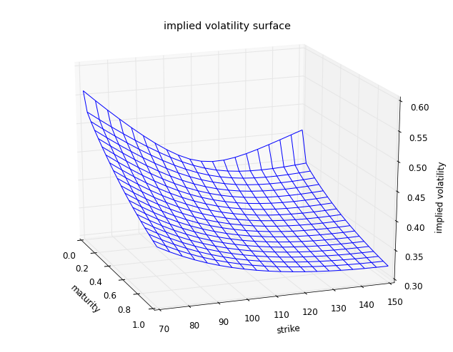
We observe that this plot reflects many of the characteristic features of real-world implied volatility surfaces for equity underlyings; see for example Fengler (2006). For short times-to-maturity, the jump component generates strongly convex implied volatility smiles. As the time-to-maturity increases, these transition into a skew shape generated by the negative correlation between the variance and spot processes. The implied volatility term structure in the example is downward sloping since the initial variance is higher than the long term level.
I implemented the implied volatility surface construction in Python and the script is attached below. It provides a minimal example of how to construct the implied volatility surface under the proposed model dynamics. The code is optimized for readability instead of performance. For practical implementations, I recommend to use the Fang and Oosterlee (2008) COS method, which exhibits better stability for out-of-the money options compared to the Carr and Madan (1999) approach. Both pricing representation can be optimized to simultaneously evaluate a vector of European plain vanilla options with different strike prices.
Attachments
- Python source code for the implied volatility surface construction: SV-ADDG.zip
References
Albrecher, Hansjörg, Philipp Mayer, Wim Schoutens and Jurgen Tistaert (2007) “The Little Heston Trap,” Wilmott Magazine, pp. 83-92
Carr, Peter P. and Dilip Madan (1999) “Option Valuation Using the Fast Fourier Transform,” Journal of Computational Finance, Vol. 2, No. 4, pp. 61-73
Cox, John C., Jonathan E. Ingersoll Jr. and Stephen A. Ross (1985) “A Theory of the Term Structure of Interest Rates,” Econometrica, Vol. 53, No. 2, pp. 385-407
Fang, Fang and Cornelis W. Oosterlee (2008) “A Novel Pricing Method for European Options Based on Fourier-Cosine Series Expansions,” SIAM Journal on Scientific Computing, Vol. 31, No. 2, pp. 826-848
Fengler, Matthias R. (2006) “Semiparametric Modelling of Implied Volatility,” Springer Finance
Heston, Steven L. (1993) “A Closed-Form Solution for Options with Stochastic Volatility with Applications to Bond and Currency Options,” Review of Financial Studies, Vol. 6, No. 2, pp. 327-343
Thul, Matthias and Ally Q. Zhang (2014) “Analytical Option Pricing under an Asymmetrically Displaced Double Gamma Jump-Diffusion Model,” Working Paper, University of New South Wales and Swiss Finance Institute